![]()
MultiNEAs: The multimin Module Tutorial
This notebook demonstrates how to use the multineas.multimin module for handling multidimensional distributions, specifically designed for asteroid population analysis.
Installation
If you’re running this in Google Colab or need to install the package, uncomment and run the following cell:
[1]:
try:
    from google.colab import drive
    %pip install -U multineas
except ImportError:
    print("Not running in Colab, skipping installation")

# Uncomment to install from GitHub (development version)
# !pip install git+https://github.com/seap-udea/MultiNEAs.git
Not running in Colab, skipping installation
Load the Package
Import multineas.multimin and other required libraries:
[2]:
import pandas as pd
import numpy as np
import multineas.multimin as mm
import warnings
%matplotlib inline

warnings.filterwarnings("ignore")
from multineas.util import Util, Stats
from multineas.plot import CornerPlot
Read data:
[5]:
df_neas=pd.read_json("data/nea_extended.json.gz")
df_neas["q"]=df_neas["a"]*(1-df_neas["e"])
data_neas=np.array(df_neas[["q","e","i"]])
Transform to unbound:
[6]:
scales=[1.35,1.00,180.0]
udata=np.zeros_like(data_neas)
for i in range(len(data_neas)):
    udata[i]=Util.t_if(data_neas[i],scales,Util.f2u)
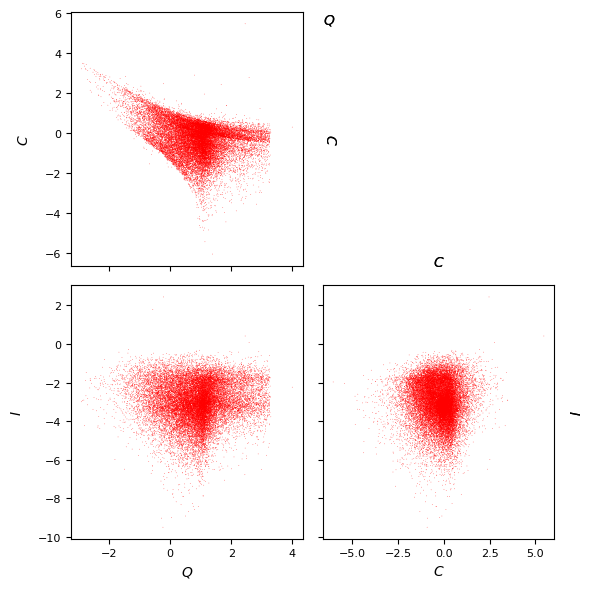
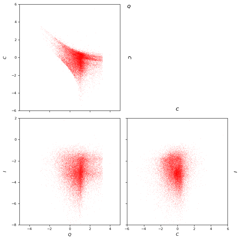
Corner plot of data:
[7]:
properties=dict(
    Q=dict(label=r"$Q$",range=None),
    E=dict(label=r"$C$",range=None),
    I=dict(label=r"$I$",range=None),
)
G=CornerPlot(properties,figsize=3)

sargs=dict(s=0.2,edgecolor='None',color='r')
hist=G.scatter_plot(udata,**sargs)
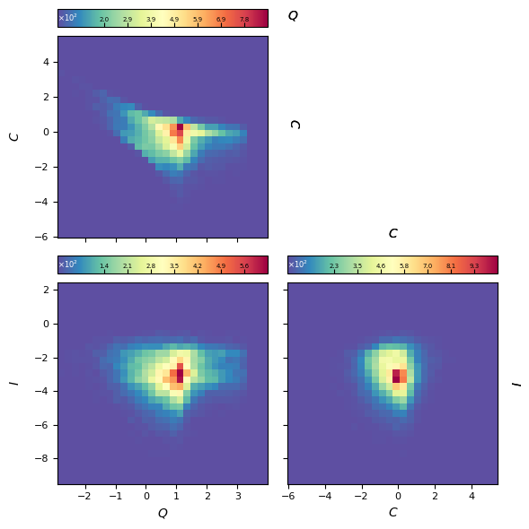
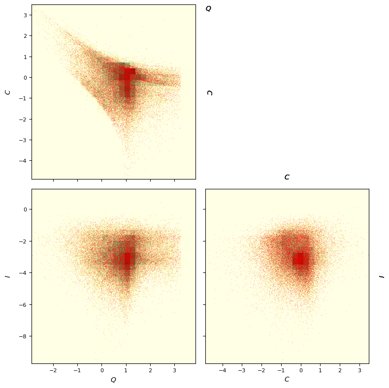
You can also make a 2-D histogram:
[8]:
G=CornerPlot(properties,figsize=3)
hargs=dict(bins=30,cmap='Spectral_r')
hist=G.plot_hist(udata,colorbar=True,**hargs)
Create a Composed multinormal:
[9]:
CMND=mm.ComposedMultiVariateNormal(Ngauss=1,Nvars=2)
print(CMND)
Composition of Ngauss = 1 gaussian multivariates of Nvars = 2 random variables:
    Weights: [1.0]
    Number of variables: 2
    Averages (μ): [[0, 0]]
    Standard deviations (σ): [[1.0, 1.0]]
    Correlation coefficients (ρ): [[0.0]]

    Covariant matrices (Σ):
        [[[1.0, 0.0], [0.0, 1.0]]]
    Flatten parameters:
        With covariance matrix (6):
            [p1,μ1_1,μ1_2,Σ1_11,Σ1_12,Σ1_22]
            [1.0, 0.0, 0.0, 1.0, 0.0, 1.0]
        With std. and correlations (6):
            [p1,μ1_1,μ1_2,σ1_1,σ1_2,ρ1_12]
            [1.0, 0.0, 0.0, 1.0, 1.0, 0.0]
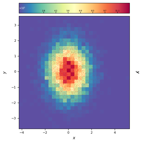
Generate a sample:
[10]:
sample = CMND.rvs(10000)
Show sample:
[11]:
properties=dict(
    x=dict(label=r"$x$",range=None),
    y=dict(label=r"$y$",range=None),
)
G=CornerPlot(properties,figsize=5)

hargs=dict(bins=30,cmap='Spectral_r')
hist=G.plot_hist(sample,colorbar=True,**hargs)

sargs=dict(s=0.2,edgecolor='None',color='r')
hist=G.scatter_plot(sample,**sargs)
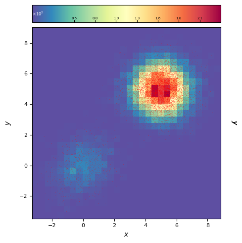
Now create a true composed distribution:
You may created specifying each parameter:
[12]:
weights=[0.1,0.9]
mus=[[0,0],[5,5]]
Sigmas=[[[1,0.2],[0,1]],[[1,0],[0,1]]]
MND=mm.ComposedMultiVariateNormal(mus=mus,weights=weights,Sigmas=Sigmas)
print(MND)
Composition of Ngauss = 2 gaussian multivariates of Nvars = 2 random variables:
    Weights: [0.1, 0.9]
    Number of variables: 2
    Averages (μ): [[0, 0], [5, 5]]
    Standard deviations (σ): [[1.0, 1.0], [1.0, 1.0]]
    Correlation coefficients (ρ): [[0.2], [0.0]]

    Covariant matrices (Σ):
        [[[1.0, 0.2], [0.2, 1.0]], [[1.0, 0.0], [0.0, 1.0]]]
    Flatten parameters:
        With covariance matrix (12):
            [p1,p2,μ1_1,μ1_2,μ2_1,μ2_2,Σ1_11,Σ1_12,Σ1_22,Σ2_11,Σ2_12,Σ2_22]
            [0.1, 0.9, 0.0, 0.0, 5.0, 5.0, 1.0, 0.2, 1.0, 1.0, 0.0, 1.0]
        With std. and correlations (12):
            [p1,p2,μ1_1,μ1_2,μ2_1,μ2_2,σ1_1,σ1_2,σ2_1,σ2_2,ρ1_12,ρ2_12]
            [0.1, 0.9, 0.0, 0.0, 5.0, 5.0, 1.0, 1.0, 1.0, 1.0, 0.2, 0.0]
Or, you may do it using a flat list of parameters:
[13]:
params=[0.1, 0.9, 0.0, 0.0, 5.0, 5.0, 1.0, 0.2, 1.0, 1.0, 0.0, 1.0]
MND=mm.ComposedMultiVariateNormal(params=params,Nvars=2)
print(MND)
Composition of Ngauss = 2 gaussian multivariates of Nvars = 2 random variables:
    Weights: [0.1, 0.9]
    Number of variables: 2
    Averages (μ): [[0.0, 0.0], [5.0, 5.0]]
    Standard deviations (σ): [[1.0, 1.0], [1.0, 1.0]]
    Correlation coefficients (ρ): [[0.2], [0.0]]

    Covariant matrices (Σ):
        [[[1.0, 0.2], [0.2, 1.0]], [[1.0, 0.0], [0.0, 1.0]]]
    Flatten parameters:
        With covariance matrix (12):
            [p1,p2,μ1_1,μ1_2,μ2_1,μ2_2,Σ1_11,Σ1_12,Σ1_22,Σ2_11,Σ2_12,Σ2_22]
            [0.1, 0.9, 0.0, 0.0, 5.0, 5.0, 1.0, 0.2, 1.0, 1.0, 0.0, 1.0]
        With std. and correlations (12):
            [p1,p2,μ1_1,μ1_2,μ2_1,μ2_2,σ1_1,σ1_2,σ2_1,σ2_2,ρ1_12,ρ2_12]
            [0.1, 0.9, 0.0, 0.0, 5.0, 5.0, 1.0, 1.0, 1.0, 1.0, 0.2, 0.0]
[14]:
sample = MND.rvs(10000)
properties=dict(
    x=dict(label=r"$x$",range=None),
    y=dict(label=r"$y$",range=None),
)
G=CornerPlot(properties,figsize=5)

hargs=dict(bins=30,cmap='Spectral_r')
hist=G.plot_hist(sample,colorbar=True,**hargs)

sargs=dict(s=0.2,edgecolor='None',color='r')
hist=G.scatter_plot(sample,**sargs)
Fitting data to a composed multinormal distribution
Create the fitting object:
[15]:
F=mm.FitCMND(Ngauss=1,Nvars=3)
The fitting object create a test CMND:
[16]:
print(F.cmnd)
Composition of Ngauss = 1 gaussian multivariates of Nvars = 3 random variables:
    Weights: [1.0]
    Number of variables: 3
    Averages (μ): [[0, 0, 0]]
    Standard deviations (σ): [[1.0, 1.0, 1.0]]
    Correlation coefficients (ρ): [[0.0, 0.0, 0.0]]

    Covariant matrices (Σ):
        [[[1.0, 0.0, 0.0], [0.0, 1.0, 0.0], [0.0, 0.0, 1.0]]]
    Flatten parameters:
        With covariance matrix (10):
            [p1,μ1_1,μ1_2,μ1_3,Σ1_11,Σ1_12,Σ1_13,Σ1_22,Σ1_23,Σ1_33]
            [1.0, 0.0, 0.0, 0.0, 1.0, 0.0, 0.0, 1.0, 0.0, 1.0]
        With std. and correlations (10):
            [p1,μ1_1,μ1_2,μ1_3,σ1_1,σ1_2,σ1_3,ρ1_12,ρ1_13,ρ1_23]
            [1.0, 0.0, 0.0, 0.0, 1.0, 1.0, 1.0, 0.0, 0.0, 0.0]
Let’s make a minimization:
[17]:
t = Util.el_time(0)
F.fit_data(udata,verbose=False,advance=1)
t = Util.el_time()
print(f"-log(L)/N = {F.solution.fun/len(udata)}")
Iterations:
Iter 0:
        Vars: [2.5, 1.7, -1.6, -1.2, -1.1, -1.5, 2.2, 1.7, 1.9]
        LogL/N: 5.482515062156635
Iter 1:
        Vars: [2.5, 1.4, -2.1, -1.3, -1.2, -1.6, 2.1, 1.8, 1.7]
        LogL/N: 5.310789889726747
Iter 2:
        Vars: [2.2, 0.87, -2.3, -1.3, -1.5, -1.7, 1.9, 1.7, 1.5]
        LogL/N: 5.113466450357126
Iter 3:
        Vars: [0.85, -0.51, -3.1, -1.9, -2.1, -1.9, 0.5, 0.78, 0.89]
        LogL/N: 4.370062348684365
Iter 4:
        Vars: [0.84, -0.45, -3, -2.2, -2.2, -2, -0.19, 0.13, 0.47]
        LogL/N: 4.122548379097678
Iter 5:
        Vars: [0.92, -0.37, -3, -2.3, -2.3, -2.1, -0.65, 0.061, -0.0057]
        LogL/N: 4.022401128011559
Iter 6:
        Vars: [0.91, -0.34, -3, -2.3, -2.3, -2.1, -0.68, 0.064, -0.061]
        LogL/N: 4.016488054693319
Iter 7:
        Vars: [0.86, -0.3, -3, -2.3, -2.4, -2.1, -0.71, 0.054, -0.083]
        LogL/N: 4.013715421099718
Iter 8:
        Vars: [0.86, -0.3, -3, -2.3, -2.4, -2.1, -0.71, 0.052, -0.074]
        LogL/N: 4.013578951513318
Iter 9:
        Vars: [0.86, -0.3, -3, -2.3, -2.4, -2.1, -0.71, 0.052, -0.074]
        LogL/N: 4.013578951513318
Elapsed time since last call: 417.098 ms
-log(L)/N = 4.013578951513318
Now you may see the result:
[18]:
print(F.cmnd)
Composition of Ngauss = 1 gaussian multivariates of Nvars = 3 random variables:
    Weights: [1.0]
    Number of variables: 3
    Averages (μ): [[0.8613186782566644, -0.2951261196561889, -3.024113027309399]]
    Standard deviations (σ): [[0.8950288462521656, 0.8641833063725712, 1.0749700951164936]]
    Correlation coefficients (ρ): [[-0.3397678420263328, 0.02610874848950706, -0.03708593257100945]]

    Covariant matrices (Σ):
        [[[0.8010766356234827, -0.2627998888091603, 0.025119990445674326], [-0.2627998888091603, 0.7468127870130293, -0.034451763693387365], [0.025119990445674326, -0.034451763693387365, 1.1555607053947632]]]
    Flatten parameters:
        With covariance matrix (10):
            [p1,μ1_1,μ1_2,μ1_3,Σ1_11,Σ1_12,Σ1_13,Σ1_22,Σ1_23,Σ1_33]
            [1.0, 0.8613186782566644, -0.2951261196561889, -3.024113027309399, 0.8010766356234827, -0.2627998888091603, 0.025119990445674326, 0.7468127870130293, -0.034451763693387365, 1.1555607053947632]
        With std. and correlations (10):
            [p1,μ1_1,μ1_2,μ1_3,σ1_1,σ1_2,σ1_3,ρ1_12,ρ1_13,ρ1_23]
            [1.0, 0.8613186782566644, -0.2951261196561889, -3.024113027309399, 0.8950288462521656, 0.8641833063725712, 1.0749700951164936, -0.3397678420263328, 0.02610874848950706, -0.03708593257100945]
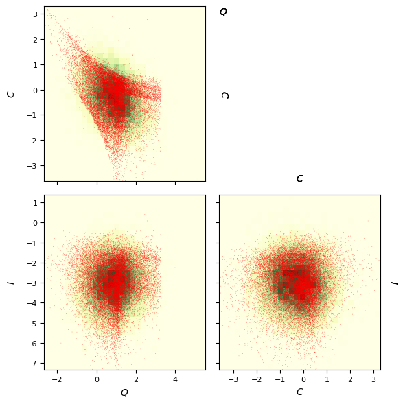
Let’s plot the fit result:_
[19]:
props=["Q","C","I"]
hargs=dict(bins=30,cmap='YlGn')
sargs=dict(s=0.2,edgecolor='None',color='r')
G=F.plot_fit(props=props,hargs=hargs,sargs=sargs,figsize=3)
Since a fitting process may be a very long process it is useful to store the result:
[20]:
F.save_fit(f"products/fit-single.pkl",useprefix=False)
If you have the result you may load it afterwards here or in another notebook:
[21]:
F=mm.FitCMND(f"products/fit-single.pkl")
print(F.cmnd)
Composition of Ngauss = 1 gaussian multivariates of Nvars = 3 random variables:
    Weights: [1.0]
    Number of variables: 3
    Averages (μ): [[0.8613186782566644, -0.2951261196561889, -3.024113027309399]]
    Standard deviations (σ): [[0.8950288462521656, 0.8641833063725712, 1.0749700951164936]]
    Correlation coefficients (ρ): [[-0.3397678420263328, 0.02610874848950706, -0.03708593257100945]]

    Covariant matrices (Σ):
        [[[0.8010766356234827, -0.2627998888091603, 0.025119990445674326], [-0.2627998888091603, 0.7468127870130293, -0.034451763693387365], [0.025119990445674326, -0.034451763693387365, 1.1555607053947632]]]
    Flatten parameters:
        With covariance matrix (10):
            [p1,μ1_1,μ1_2,μ1_3,Σ1_11,Σ1_12,Σ1_13,Σ1_22,Σ1_23,Σ1_33]
            [1.0, 0.8613186782566644, -0.2951261196561889, -3.024113027309399, 0.8010766356234827, -0.2627998888091603, 0.025119990445674326, 0.7468127870130293, -0.034451763693387365, 1.1555607053947632]
        With std. and correlations (10):
            [p1,μ1_1,μ1_2,μ1_3,σ1_1,σ1_2,σ1_3,ρ1_12,ρ1_13,ρ1_23]
            [1.0, 0.8613186782566644, -0.2951261196561889, -3.024113027309399, 0.8950288462521656, 0.8641833063725712, 1.0749700951164936, -0.3397678420263328, 0.02610874848950706, -0.03708593257100945]
Let’s try with two MND:
[22]:
F=mm.FitCMND(Ngauss=2,Nvars=3)

Util.el_time(0)
F.fit_data(udata,advance=5)
Util.el_time()
F.save_fit(f"products/fit-multiple.pkl",useprefix=False)

print(f"-log(L)/N = {F.solution.fun/len(udata)}")
print(F.cmnd)

G=F.plot_fit(figsize=4,
            props=["Q","C","I"],
            hargs=dict(bins=30,cmap='YlGn'),sargs=dict(s=0.2,edgecolor='None',color='r'))
F.fig.savefig(f"products/fit-multiple-{F.prefix}.png")
Iterations:
Iter 0:
        Vars: [0.5, 0.5, 2.6, 1.8, -1.6, 2.5, 1.7, -1.6, -1.2, -1.1, -1.6, -1.4, -1.2, -1.5, 2.7, 1.7, 2, 1.6, 1.7, 1.7]
        LogL/N: 5.426799049658642
Iter 5:
        Vars: [-1.2, 0.48, 1, -0.29, -3.3, 0.82, -0.31, -2.9, -3.3, -2.8, -2.1, -2.2, -2.2, -2.1, -0.11, 0.44, -0.66, -0.76, 0.041, 0.12]
        LogL/N: 3.9682000280743477
Iter 10:
        Vars: [-1.2, 0.47, 1.2, 0.069, -3.7, 0.65, -0.37, -2.8, -2.4, -3.4, -2.1, -2.4, -2.3, -2.3, -0.78, 0.89, -0.027, -1.1, 0.077, 0.19]
        LogL/N: 3.905112231099651
Iter 15:
        Vars: [-0.43, 0.48, 1.4, 0.02, -3.3, 0.48, -0.43, -2.8, -2.5, -3.2, -2.1, -2.4, -2.2, -2.2, -0.98, 0.83, -0.31, -1.5, 0.032, 0.18]
        LogL/N: 3.874072798667041
Iter 17:
        Vars: [-0.24, 0.48, 1.4, 0.013, -3.3, 0.48, -0.46, -2.8, -2.5, -3.2, -2.1, -2.4, -2.2, -2.2, -0.92, 0.77, -0.3, -1.5, 0.019, 0.2]
        LogL/N: 3.873027386227566
Elapsed time since last call: 3.07424 s
-log(L)/N = 3.873027386227566
Composition of Ngauss = 2 gaussian multivariates of Nvars = 3 random variables:
    Weights: [0.4158221388802772, 0.5841778611197227]
    Number of variables: 3
    Averages (μ): [[1.3543152311877784, 0.012735060825352603, -3.32612391029033], [0.4823847698957606, -0.46030893323150046, -2.804584331921477]]
    Standard deviations (σ): [[0.7602640748595322, 0.40122582381564603, 1.0789725108332942], [0.8108925747517383, 1.0286081661962714, 1.0199222717987626]]
    Correlation coefficients (ρ): [[-0.4306950594759848, 0.36536218346680993, -0.14682729660458482], [-0.6458184881826532, 0.009504121964859724, 0.1016566166530517]]

    Covariant matrices (Σ):
        [[[0.5780014635220203, -0.13137817855410974, 0.299708074338082], [-0.13137817855410974, 0.16098216169654384, -0.06356324496722943], [0.299708074338082, -0.06356324496722943, 1.164181679133903]], [[0.6575467677875034, -0.5386712105730234, 0.007860359332050504], [-0.5386712105730234, 1.0580347595656563, 0.10664799492211653], [0.007860359332050504, 0.10664799492211653, 1.040241440511149]]]
    Flatten parameters:
        With covariance matrix (20):
            [p1,p2,μ1_1,μ1_2,μ1_3,μ2_1,μ2_2,μ2_3,Σ1_11,Σ1_12,Σ1_13,Σ1_22,Σ1_23,Σ1_33,Σ2_11,Σ2_12,Σ2_13,Σ2_22,Σ2_23,Σ2_33]
            [0.439281512938924, 0.6171353342299593, 1.3543152311877784, 0.012735060825352603, -3.32612391029033, 0.4823847698957606, -0.46030893323150046, -2.804584331921477, 0.5780014635220203, -0.13137817855410974, 0.299708074338082, 0.16098216169654384, -0.06356324496722943, 1.164181679133903, 0.6575467677875034, -0.5386712105730234, 0.007860359332050504, 1.0580347595656563, 0.10664799492211653, 1.040241440511149]
        With std. and correlations (20):
            [p1,p2,μ1_1,μ1_2,μ1_3,μ2_1,μ2_2,μ2_3,σ1_1,σ1_2,σ1_3,σ2_1,σ2_2,σ2_3,ρ1_12,ρ1_13,ρ1_23,ρ2_12,ρ2_13,ρ2_23]
            [0.439281512938924, 0.6171353342299593, 1.3543152311877784, 0.012735060825352603, -3.32612391029033, 0.4823847698957606, -0.46030893323150046, -2.804584331921477, 0.7602640748595322, 0.40122582381564603, 1.0789725108332942, 0.8108925747517383, 1.0286081661962714, 1.0199222717987626, -0.43069505947598485, 0.36536218346680993, -0.14682729660458482, -0.6458184881826532, 0.009504121964859724, 0.1016566166530517]
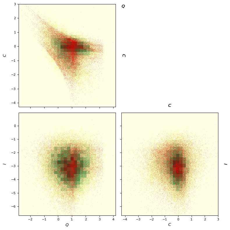
Notice that by using two multinormals you now obtain a better value of the \(\log {\cal L}\).
You can also fit setting bounds in parameters to avoid divergences:
[23]:
F=mm.FitCMND(Ngauss=2,Nvars=3)
bounds=F.set_bounds(boundsm=((-2,4),(-4,3),(-7,0)),boundw=(0.1,0.9))

Util.el_time(0)
F.fit_data(udata,advance=5,bounds=bounds)
Util.el_time()
F.save_fit(f"products/fit-multiple-bounds.pkl",useprefix=False)

print(f"-log(L)/N = {F.solution.fun/len(udata)}")
print(F.cmnd)
G=F.plot_fit(figsize=4,
            props=["Q","C","I"],
            hargs=dict(bins=30,cmap='YlGn'),sargs=dict(s=0.2,edgecolor='None',color='r'))
F.fig.savefig(f"products/fit-multiple-bounds-{F.prefix}.png")
Iterations:
Iter 0:
        Vars: [2.2, 2.2, 2.6, 1.8, -1.6, 2.5, 1.7, -1.6, -1.3, -1.1, -1.6, -1.4, -1.2, -1.5, 2.7, 1.7, 2, 1.6, 1.7, 1.7]
        LogL/N: 5.424820534630294
Iter 5:
        Vars: [2.1, 0.85, 1.1, -0.44, -3, 0.5, -0.048, -3.1, -2.5, -2.6, -2.3, -2.3, -2.2, -1.9, -0.029, 0.36, -0.63, -1.2, -0.32, 0.32]
        LogL/N: 3.961435153174314
Iter 10:
        Vars: [1.7, -0.13, 1.2, -0.23, -3, 0.11, -0.16, -3, -2.5, -2.8, -2.2, -2.5, -2, -2, -0.34, 0.32, -0.48, -1.9, -0.31, 0.16]
        LogL/N: 3.9058015702390967
Iter 15:
        Vars: [-0.1, -0.46, 1.3, -0.16, -3.3, 0.35, -0.42, -2.7, -2.5, -2.9, -2.1, -2.4, -2, -2.3, -0.48, 0.69, -0.25, -1.8, -0.068, 0.29]
        LogL/N: 3.8857335749186324
Iter 20:
        Vars: [-1.4, -0.99, 1.4, -0.0069, -3.3, 0.5, -0.48, -2.8, -2.5, -3.1, -2.1, -2.5, -2.2, -2.2, -0.9, 0.79, -0.31, -1.5, -0.0038, 0.24]
        LogL/N: 3.875229773397918
Iter 23:
        Vars: [-1.6, -0.97, 1.4, 0.045, -3.3, 0.53, -0.47, -2.8, -2.5, -3.2, -2.1, -2.4, -2.2, -2.2, -1, 0.81, -0.3, -1.5, 0.027, 0.19]
        LogL/N: 3.8723569871930104
Elapsed time since last call: 4.15155 s
-log(L)/N = 3.8723569871930104
Composition of Ngauss = 2 gaussian multivariates of Nvars = 3 random variables:
    Weights: [0.3808162405996863, 0.6191837594003137]
    Number of variables: 3
    Averages (μ): [[1.3785085843355145, 0.04518318316509815, -3.3437473064063092], [0.5299511746669845, -0.47342618399748737, -2.819824580067435]]
    Standard deviations (σ): [[0.7750237601135864, 0.3832547894948384, 1.0786079938235054], [0.8066020815866669, 1.0050091568900978, 1.0241023284407793]]
    Correlation coefficients (ρ): [[-0.47905226460480066, 0.383907763335426, -0.15055468645641779], [-0.6239746275132241, 0.013692056464986058, 0.0969244409841985]]

    Covariant matrices (Σ):
        [[[0.6006618287406019, -0.14229364532667962, 0.32092647510895894], [-0.14229364532667962, 0.1468842336707329, -0.06223654916205823], [0.32092647510895894, -0.06223654916205823, 1.163395204339967]], [[0.6506069180199441, -0.5058203382322455, 0.011310228355281164], [-0.5058203382322455, 1.0100434054329452, 0.09975775734112025], [0.011310228355281164, 0.09975775734112025, 1.0487855791178258]]]
    Flatten parameters:
        With covariance matrix (20):
            [p1,p2,μ1_1,μ1_2,μ1_3,μ2_1,μ2_2,μ2_3,Σ1_11,Σ1_12,Σ1_13,Σ1_22,Σ1_23,Σ1_33,Σ2_11,Σ2_12,Σ2_13,Σ2_22,Σ2_23,Σ2_33]
            [0.16884223164952697, 0.27452707262080683, 1.3785085843355145, 0.04518318316509815, -3.3437473064063092, 0.5299511746669845, -0.47342618399748737, -2.819824580067435, 0.6006618287406019, -0.14229364532667962, 0.32092647510895894, 0.1468842336707329, -0.06223654916205823, 1.163395204339967, 0.6506069180199441, -0.5058203382322455, 0.011310228355281164, 1.0100434054329452, 0.09975775734112025, 1.0487855791178258]
        With std. and correlations (20):
            [p1,p2,μ1_1,μ1_2,μ1_3,μ2_1,μ2_2,μ2_3,σ1_1,σ1_2,σ1_3,σ2_1,σ2_2,σ2_3,ρ1_12,ρ1_13,ρ1_23,ρ2_12,ρ2_13,ρ2_23]
            [0.16884223164952697, 0.27452707262080683, 1.3785085843355145, 0.04518318316509815, -3.3437473064063092, 0.5299511746669845, -0.47342618399748737, -2.819824580067435, 0.7750237601135864, 0.3832547894948384, 1.0786079938235054, 0.8066020815866669, 1.0050091568900978, 1.0241023284407793, -0.47905226460480066, 0.383907763335426, -0.15055468645641779, -0.6239746275132241, 0.013692056464986058, 0.0969244409841985]
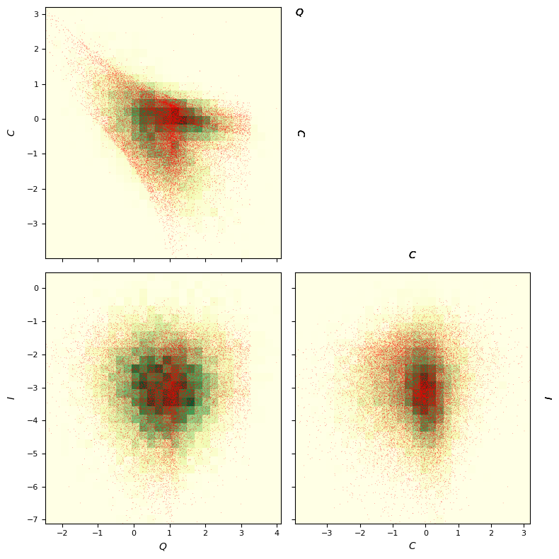
Five gaussians:
[24]:
F=mm.FitCMND(Ngauss=5,Nvars=3)
bounds=F.set_bounds(boundsm=((-2,4),(-4,3),(-7,0)),boundw=(0.1,0.9))

Util.el_time(0)
F.fit_data(udata,advance=10,bounds=bounds)
Util.el_time()
F.save_fit(f"products/fit-multiple-bound_mus.pkl",useprefix=False)

print(f"-log(L)/N = {F.solution.fun/len(udata)}")
print(F.cmnd)
G=F.plot_fit(figsize=4,
            props=["Q","C","I"],
            hargs=dict(bins=30,cmap='YlGn'),sargs=dict(s=0.2,edgecolor='None',color='r'))
F.fig.savefig(f"products/fit-multiple-bound_mus-{F.prefix}.png")
Iterations:
Iter 0:
        Vars: [2.2, 2.2, 2.2, 2.2, 2.2, 2.6, 1.8, -1.7, 2.6, 1.7, -1.7, 2.6, 1.7, -1.6, 2.5, 1.7, -1.6, 2.5, 1.7, -1.6, -1.3, -1.2, -1.7, -1.4, -1.2, -1.6, -1.4, -1.3, -1.6, -1.4, -1.3, -1.5, -1.4, -1.3, -1.4, 3.5, 1.7, 1.9, 2.3, 2.2, 2.1, 1.8, 1.9, 1.9, 1.6, 1.6, 1.8, 1.6, 1.6, 1.6]
        LogL/N: 5.406394477165358
Iter 10:
        Vars: [-0.97, 1.1, 0.14, -0.78, -0.12, 2, 0.028, -2.9, 0.99, -0.54, -2.9, 0.62, 0.38, -3.4, 1.5, -0.93, -3.4, -0.18, -0.31, -2.6, -2.7, -3.6, -2.5, -3.2, -2.8, -2.3, -2.7, -3.2, -2.1, -2.5, -2.5, -1.8, -2.5, -1.9, -2.3, -1, -0.032, 0.7, -0.31, 0.46, -0.46, -1.9, -0.19, 0.23, -0.0011, 1.5, -0.15, -2.7, -0.28, 0.44]
        LogL/N: 3.770311933388413
Iter 18:
        Vars: [-0.18, 0.46, -0.73, -0.95, 0.32, 1.5, 0.091, -3.1, 1, -0.56, -2.8, 0.7, 0.49, -3.5, 1.5, -0.8, -3.6, 0.015, -0.48, -2.6, -2.3, -3.6, -2.4, -3.3, -2.8, -2.3, -2.6, -3.2, -2, -2.4, -2.6, -1.8, -2.5, -2, -2.3, -0.99, 0.51, 0.37, -0.65, 0.63, -0.39, -2.7, -0.053, 0.22, -0.17, 1.7, -0.17, -2.4, -0.17, 0.41]
        LogL/N: 3.760765705868478
Elapsed time since last call: 18.9497 s
-log(L)/N = 3.760765705868478
Composition of Ngauss = 5 gaussian multivariates of Nvars = 3 random variables:
    Weights: [0.20173431512632206, 0.27230238807490303, 0.14493777167039407, 0.12360741432303296, 0.25741811080534777]
    Number of variables: 3
    Averages (μ): [[1.4525217633416425, 0.09114259008830537, -3.130053063589653], [1.014376591283622, -0.5584925884515662, -2.82642119892797], [0.6970423954033862, 0.4903676096572116, -3.5156796774801986], [1.4890864424380457, -0.7955631890742869, -3.5537761048491845], [0.014744956576950003, -0.48132811233434025, -2.61044142970533]]
    Standard deviations (σ): [[0.8713627405395032, 0.2767092303299922, 0.823247841910546], [0.3639029857702276, 0.5631278623408879, 0.888119693602703], [0.7053279496809249, 0.3982431653810926, 1.16707568135325], [0.8085738648706087, 0.719943855548447, 1.4790307568683208], [0.7495114603031392, 1.2138601949489074, 0.9024375820224185]]
    Correlation coefficients (ρ): [[-0.4594427038883665, 0.24884743088322558, 0.18354994823689919], [-0.3138164948816674, 0.30359173712908283, -0.1922518280093921], [-0.8764505271893462, -0.026441712680007497, 0.11037235825930325], [-0.08670179503979092, 0.6887085660633578, -0.08305282810210246], [-0.8362467099943731, -0.08281861336837393, 0.20247751881931686]]

    Covariant matrices (Σ):
        [[[0.7592730256005137, -0.11077812014775561, 0.1785100813480961], [-0.11077812014775561, 0.07656799814981666, 0.0418127289977182], [0.1785100813480961, 0.0418127289977182, 0.6777370092103714]], [[0.1324253830524865, -0.06430850330310288, 0.09811763386425117], [-0.06430850330310288, 0.31711298934461796, -0.09614993482501244], [0.09811763386425117, -0.09614993482501244, 0.7887565901649591]], [[0.49748751660109736, -0.24618797243309348, -0.021766053645295214], [-0.24618797243309348, 0.15859761877275227, 0.05129885513353579], [-0.021766053645295214, 0.05129885513353579, 1.3620656460061524]], [[0.6537916949517933, -0.05047152396885464, 0.823630441490353], [-0.05047152396885464, 0.5183191551419631, -0.08843623813511481], [0.823630441490353, -0.08843623813511481, 2.1875319797624777]], [[0.5617674291257442, -0.7608190357172392, -0.056017459108703156], [-0.7608190357172392, 1.4734565728813995, 0.22180056786816696], [-0.056017459108703156, 0.22180056786816696, 0.8143935894464693]]]
    Flatten parameters:
        With covariance matrix (50):
            [p1,p2,p3,p4,p5,μ1_1,μ1_2,μ1_3,μ2_1,μ2_2,μ2_3,μ3_1,μ3_2,μ3_3,μ4_1,μ4_2,μ4_3,μ5_1,μ5_2,μ5_3,Σ1_11,Σ1_12,Σ1_13,Σ1_22,Σ1_23,Σ1_33,Σ2_11,Σ2_12,Σ2_13,Σ2_22,Σ2_23,Σ2_33,Σ3_11,Σ3_12,Σ3_13,Σ3_22,Σ3_23,Σ3_33,Σ4_11,Σ4_12,Σ4_13,Σ4_22,Σ4_23,Σ4_33,Σ5_11,Σ5_12,Σ5_13,Σ5_22,Σ5_23,Σ5_33]
            [0.4539985021788449, 0.6128103503279404, 0.3261791689048772, 0.2781756833274356, 0.5793136218107253, 1.4525217633416425, 0.09114259008830537, -3.130053063589653, 1.014376591283622, -0.5584925884515662, -2.82642119892797, 0.6970423954033862, 0.4903676096572116, -3.5156796774801986, 1.4890864424380457, -0.7955631890742869, -3.5537761048491845, 0.014744956576950003, -0.48132811233434025, -2.61044142970533, 0.7592730256005137, -0.11077812014775561, 0.1785100813480961, 0.07656799814981666, 0.0418127289977182, 0.6777370092103714, 0.1324253830524865, -0.06430850330310288, 0.09811763386425117, 0.31711298934461796, -0.09614993482501244, 0.7887565901649591, 0.49748751660109736, -0.24618797243309348, -0.021766053645295214, 0.15859761877275227, 0.05129885513353579, 1.3620656460061524, 0.6537916949517933, -0.05047152396885464, 0.823630441490353, 0.5183191551419631, -0.08843623813511481, 2.1875319797624777, 0.5617674291257442, -0.7608190357172392, -0.056017459108703156, 1.4734565728813995, 0.22180056786816696, 0.8143935894464693]
        With std. and correlations (50):
            [p1,p2,p3,p4,p5,μ1_1,μ1_2,μ1_3,μ2_1,μ2_2,μ2_3,μ3_1,μ3_2,μ3_3,μ4_1,μ4_2,μ4_3,μ5_1,μ5_2,μ5_3,σ1_1,σ1_2,σ1_3,σ2_1,σ2_2,σ2_3,σ3_1,σ3_2,σ3_3,σ4_1,σ4_2,σ4_3,σ5_1,σ5_2,σ5_3,ρ1_12,ρ1_13,ρ1_23,ρ2_12,ρ2_13,ρ2_23,ρ3_12,ρ3_13,ρ3_23,ρ4_12,ρ4_13,ρ4_23,ρ5_12,ρ5_13,ρ5_23]
            [0.4539985021788449, 0.6128103503279404, 0.3261791689048772, 0.2781756833274356, 0.5793136218107253, 1.4525217633416425, 0.09114259008830537, -3.130053063589653, 1.014376591283622, -0.5584925884515662, -2.82642119892797, 0.6970423954033862, 0.4903676096572116, -3.5156796774801986, 1.4890864424380457, -0.7955631890742869, -3.5537761048491845, 0.014744956576950003, -0.48132811233434025, -2.61044142970533, 0.8713627405395032, 0.2767092303299922, 0.823247841910546, 0.3639029857702276, 0.5631278623408879, 0.888119693602703, 0.7053279496809249, 0.3982431653810926, 1.16707568135325, 0.8085738648706087, 0.719943855548447, 1.4790307568683208, 0.7495114603031392, 1.2138601949489074, 0.9024375820224185, -0.4594427038883665, 0.24884743088322558, 0.18354994823689919, -0.3138164948816674, 0.30359173712908283, -0.1922518280093921, -0.8764505271893462, -0.0264417126800075, 0.11037235825930325, -0.08670179503979092, 0.6887085660633578, -0.08305282810210246, -0.8362467099943731, -0.08281861336837393, 0.20247751881931686]
As you can see the fitting parameter \(-\log{\cal L}\) is improved with respect to previous fit.
You can verify that the fit is capturing the details of the distribution by generating and plotting a mock distribution:
[25]:
F.cmnd.plot_sample(N=len(F.data),
                  figsize=4,
                  props=["Q","C","I"],ranges=[[-5,5],[-6,6],[-8,2]],
                  sargs=dict(s=0.2,edgecolor='None',color='r'))
G.fig.savefig(f"products/sample-multiple-{F.prefix}.png")

Compare this with the original distribution:
[26]:
properties=dict(
    Q=dict(label=r"$Q$",range=[-5,5]),
    C=dict(label=r"$C$",range=[-6,6]),
    I=dict(label=r"$I$",range=[-8,2]),
)
G=CornerPlot(properties,figsize=4)
sargs=dict(s=0.2,edgecolor='None',color='r')
hist=G.scatter_plot(udata,**sargs)
G.fig.savefig("products/true-MPCsample.png")
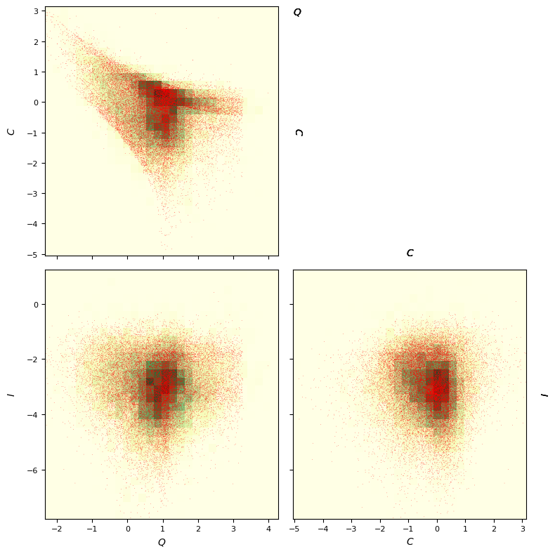
Let’s try with 20 MND:
[27]:
F=mm.FitCMND(Ngauss=20,Nvars=3)
bounds=F.set_bounds(boundsm=((-2,4),(-4,3),(-7,0)),boundw=(0.1,0.9))

Util.el_time(0)
F.fit_data(udata,advance=10,bounds=bounds)
Util.el_time()
F.save_fit(f"products/fit-multiple-bound_mus.pkl",useprefix=True)

print(f"-log(L)/N = {F.solution.fun/len(udata)}")
print(F.cmnd)
G=F.plot_fit(figsize=4,
            props=["Q","C","I"],
            hargs=dict(bins=30,cmap='YlGn'),sargs=dict(s=0.2,edgecolor='None',color='r'))
F.fig.savefig(f"products/fit-multiple-bound_mus-{F.prefix}.png")
Iterations:
Iter 0:
        Vars: [1.8, 2, 0.53, 2.1, 2.2, 1, -0.4, 2.2, 2.2, 1, 1.8, 2.2, 0.52, 1.8, 2.2, 2.2, 2.2, 2.2, 2.2, 2.2, 2.6, 1.8, -1.7, 2.6, 1.8, -1.7, 2.6, 1.8, -1.7, 2.6, 1.8, -1.7, 2.6, 1.7, -1.7, 2.6, 1.7, -1.7, 2.6, 1.7, -1.7, 2.6, 1.7, -1.7, 2.6, 1.7, -1.7, 2.6, 1.7, -1.7, 2.6, 1.7, -1.7, 2.6, 1.7, -1.6, 2.6, 1.7, -1.6, 2.6, 1.7, -1.6, 2.5, 1.7, -1.6, 2.5, 1.7, -1.6, 2.5, 1.7, -1.6, 2.5, 1.7, -1.6, 2.5, 1.7, -1.6, 2.5, 1.7, -1.6, -1.4, -1.2, -1.9, -1.4, -1.3, -1.8, -1.4, -1.3, -1.8, -1.4, -1.3, -1.7, -1.4, -1.3, -1.7, -1.4, -1.3, -1.7, -1.4, -1.3, -1.6, -1.4, -1.3, -1.6, -1.4, -1.3, -1.6, -1.4, -1.3, -1.6, -1.4, -1.3, -1.6, -1.4, -1.3, -1.6, -1.4, -1.3, -1.6, -1.4, -1.3, -1.6, -1.4, -1.3, -1.5, -1.4, -1.3, -1.5, -1.4, -1.3, -1.9, -1.4, -1.4, -1.2, -1.4, -1.3, -3.3, -1.4, -1.4, -1.1, 4.7, 1.6, 1.7, 3.6, 1.8, 2.1, 3.2, 2, 2.3, 2.9, 2.2, 2.4, 2.6, 2.4, 2.4, 2.4, 2.6, 2.3, 2.4, 2.6, 2.3, 2.1, 2.4, 2.1, 1.9, 2.1, 2, 1.8, 1.9, 2, 1.6, 1.7, 1.9, 1.6, 1.7, 1.9, 1.8, 1.8, 1.9, 1.5, 1.5, 1.8, 1.7, 1.8, 1.8, 1.6, 1.7, 1.7, 1.2, 1.2, 1.4, 3, 1.8, 1.9, 1.2, 0.83, 1.3, 2, 1.9, 1.9]
        LogL/N: 5.385236332947701
Iter 10:
        Vars: [-1.1, 2.1, -1.8, 2.1, -1.8, 0.52, 2.2, 2.2, 0.43, 0.78, 1.6, -0.22, 0.06, 1.9, 1.8, -0.64, -0.52, -2, 2.2, -2.2, -0.47, 1.1, -2.9, 1.6, -0.85, -2.1, -1.5, 1.8, -2.3, 0.95, -1.3, -3.5, 1.5, -1.4, -4.5, 2.4, -0.16, -3.2, 1.5, 0.015, -3.2, 1.1, -0.5, -3.3, 1, -0.46, -2.5, 1, 0.05, -3.2, 0.59, 0.56, -3.1, 0.092, 0.5, -3.8, -0.61, -0.14, -2.8, 0.24, -0.74, -3, 1.1, 0.28, -3.7, 1, -1.9, -3.8, 0.41, -0.12, -2.8, -0.88, 1.6, -2.8, 0.62, -0.7, -1.8, 0.28, 0.18, -4.5, -3.4, -3.9, -2.3, -2.5, -2.8, -2.8, -2.9, -2.6, -2.4, -3.2, -2.8, -2.2, -2.4, -2.3, -1.6, -3.1, -3.4, -2.5, -2.6, -3.8, -2.4, -3.9, -3.2, -2.2, -3.2, -2.9, -2.6, -2.8, -3.6, -3.4, -3, -3.6, -2.3, -3.1, -3.5, -2, -3.2, -2.8, -2.3, -3.4, -2.9, -2.3, -3.4, -4, -2, -3.9, -2.1, -2, -2.8, -3, -2.5, -3.4, -3.6, -2.2, -2.5, -2.3, -3.1, -2.3, -2.2, -1.4, -0.91, 0.022, -0.18, -0.17, 0.55, 0.64, -2.2, 0.36, -0.4, 0.21, 0.88, -0.82, -0.54, 1.4, -1.2, -0.2, 0.19, 0.34, -0.085, 1.2, 1.1, -0.76, 0.4, -0.5, 0.6, 1.2, 0.28, -1.5, 0.12, -0.72, -1.8, -0.00082, 0.31, -1.2, -0.7, -0.18, -2.4, -0.16, 0.43, -0.75, 0.27, -0.18, -0.37, 0.3, 0.38, -0.32, 0.87, -0.55, -2.4, -0.5, 0.63, -3.1, -0.49, 0.79, -1.6, -0.36, 1, -0.49, 0.055, 1.1]
        LogL/N: 3.693709544124691
Iter 20:
        Vars: [-1.6, 2.2, -1.9, 2.1, -2.1, -0.73, 2.2, 1.6, 2.2, 0.1, 0.23, 0.75, -1, 0.35, 0.24, -1.9, 2.2, -1.9, 2.2, -2.2, -0.41, 1.1, -2.8, 1.7, -0.7, -2, -1.4, 1.6, -2.2, 0.83, -1.2, -3.4, 1.2, -1.5, -4.9, 2.7, -0.1, -3, 1.4, 0.089, -3.3, 1.1, -0.63, -3.6, 0.85, -0.43, -2.8, 1.5, -0.04, -3.2, 0.64, 0.56, -3, 0.24, 0.49, -3.7, -0.58, -0.38, -2.9, 0.11, -0.98, -3, 1.1, 0.35, -3.5, 1, -2.4, -4.1, 0.71, -0.15, -3.1, -0.88, 1.6, -2.8, 0.48, -0.58, -1.8, 0.72, 0.085, -3.9, -3.4, -3.9, -2.5, -2.6, -2.7, -2.9, -2.7, -2.4, -2.5, -3.3, -2.6, -2.2, -2.6, -2.2, -1.6, -3.4, -3.6, -2.4, -2.6, -3.7, -2.3, -4, -2.9, -2.1, -3.1, -3.1, -2.5, -2.6, -3.9, -3.7, -3, -3.6, -2.4, -2.8, -3.3, -2, -3.4, -3.1, -2.3, -3.4, -2.7, -2.2, -3.6, -4.3, -2.1, -4.1, -2.1, -1.9, -2.4, -2.9, -2.8, -3.1, -3.3, -2.2, -2.5, -2.3, -3.1, -2, -2.1, -1.6, -1.4, 0.37, -0.23, -0.41, 0.33, 0.44, -2.5, 0.57, -0.58, -0.75, 1.1, -0.84, -1, 1.9, -1.5, -0.31, 0.094, 0.38, -0.0049, 0.93, 0.8, -0.83, 0.72, -0.64, -0.032, 0.85, -0.31, -2.6, -0.18, 0.23, -1.8, 0.31, 0.25, -2, -0.54, 0.13, -3, -0.042, 0.21, -2.2, 0.25, -0.00069, -1.2, 0.17, -0.015, -1.1, 1, -1, -1.7, -0.56, 0.0039, -3.6, -0.64, 0.84, -2, -0.45, 0.97, -0.93, 0.1, 0.79]
        LogL/N: 3.6759034723730406
Iter 24:
        Vars: [-2, 1.7, -2.1, 1.2, -1.7, -1.1, 2.2, 1.2, 1.6, -0.33, 0.2, 0.59, -1.1, 0.018, -0.57, -2.2, 2.2, -2, 2.2, -2.2, -0.39, 1.1, -2.9, 1.6, -0.68, -2, -1.4, 1.5, -2.2, 0.84, -1.2, -3.4, 1, -1.3, -4.9, 2.8, -0.11, -2.9, 1.5, 0.13, -3.3, 1.1, -0.6, -3.5, 0.8, -0.43, -2.9, 1.6, -0.071, -3.2, 0.62, 0.55, -2.9, 0.31, 0.48, -3.8, -0.54, -0.42, -2.9, 0.14, -1.1, -3.3, 1.1, 0.37, -3.6, 1, -2.5, -4.1, 0.81, -0.15, -3.1, -0.87, 1.6, -2.9, 0.41, -0.51, -1.8, 0.97, -0.2, -3.6, -3.4, -4, -2.6, -2.5, -2.7, -3, -2.6, -2.3, -2.5, -3.4, -2.6, -2.3, -2.9, -2.2, -1.7, -3.6, -3.6, -2.3, -2.6, -3.8, -2.3, -4, -3, -2.1, -3.1, -3, -2.5, -2.6, -4, -3.7, -2.9, -3.6, -2.5, -2.6, -3.2, -2, -3.4, -3.1, -2.3, -3.4, -2.7, -2.1, -3.8, -4.3, -2.1, -4.1, -2.1, -1.9, -2.4, -3, -2.8, -3, -3.3, -2.2, -2.4, -2.2, -3, -2, -2, -1.7, -1.5, 0.31, -0.14, -0.48, 0.16, 0.53, -2.7, 0.48, -0.48, -0.92, 0.93, -1.1, -1.1, 1.8, -1.3, -0.21, 0.036, 0.36, -0.2, 0.82, 0.56, -0.82, 0.72, -0.5, -0.42, 0.75, -0.68, -2.6, -0.34, 0.39, -1.6, 0.44, 0.2, -2.2, -0.64, 0.27, -3, 0.22, -0.03, -2.2, 0.17, 0.069, -1.5, 0.27, -0.18, -1.1, 0.99, -1.1, -1.5, -0.42, -0.22, -3.7, -0.71, 0.89, -2.1, -0.38, 0.85, -1.1, 0.23, 0.51]
        LogL/N: 3.673463650178416
Elapsed time since last call: 6.7668 min
-log(L)/N = 3.673463650178416
Composition of Ngauss = 20 gaussian multivariates of Nvars = 3 random variables:
    Weights: [0.012565603625617011, 0.0881262364043709, 0.011540815970877784, 0.08050232937795376, 0.01545796076907111, 0.02555780913115173, 0.0937422176778212, 0.08078821073860719, 0.08720652992911102, 0.04344302124617415, 0.05727723119423558, 0.0671294551185946, 0.02507103676559199, 0.05254196954396682, 0.03772343839080215, 0.010534785113030057, 0.09374249735607948, 0.012902602613104733, 0.09373006072131275, 0.010416188312526125]
    Number of variables: 3
    Averages (μ): [[-0.393380553865179, 1.1343947139869446, -2.8710004605621338], [1.6108551457527762, -0.678600059340867, -1.9620601780427689], [-1.3629026048130848, 1.479607326184627, -2.2485666535249775], [0.8350923884286169, -1.2328953841659684, -3.350603505109695], [1.01884487615166, -1.292500632782613, -4.921457073415205], [2.789753501832656, -0.1090868657191523, -2.9449861027121567], [1.4674442828095464, 0.12725130091670064, -3.2716544360166435], [1.1114030790302416, -0.599852301228318, -3.506628387192499], [0.7967805737492597, -0.4347626595111422, -2.925438575195619], [1.5906778200474472, -0.07103487116954674, -3.1852085111076045], [0.6180121632327902, 0.5508811383830549, -2.9055104194015944], [0.3105946008658186, 0.4831091462553804, -3.807881413401972], [-0.5416315252978482, -0.4236290296735867, -2.9032464644794054], [0.1420466564468278, -1.0698785314121804, -3.262518065512812], [1.0981841813526325, 0.36681830104985624, -3.6325253202815535], [1.002978580154458, -2.4962732750115557, -4.130998619669692], [0.8131779080633712, -0.15443118849383344, -3.0991746671043927], [-0.8734362983669943, 1.6113540371136656, -2.859962487882722], [0.40880883386166394, -0.509023338134674, -1.8182379249102067], [0.9673319554401504, -0.2026537161756422, -3.5819176171836067]]
    Standard deviations (σ): [[0.3125102921404776, 0.17673606072879955, 0.6917920624091051], [0.7321547661776288, 0.6139689570723035, 0.4918475601017075], [0.6627525839333503, 0.877465236651825, 0.7346585060440164], [0.32500652555369935, 0.7136066974826845, 0.9191648771998057], [0.546371717437319, 0.9548872651424937, 1.601502820162272], [0.2739464637371154, 0.26844380731710693, 0.8758441190139798], [0.6634245693488455, 0.22374711189762997, 0.939625473734322], [0.17526850953388523, 0.4890150932388802, 1.0533092632950247], [0.44128392757268897, 0.48504432984698725, 0.743717936197336], [0.6842266190005744, 0.18015118871785932, 0.24654320515635805], [0.5441064048234064, 0.2546074687085019, 0.7850461925271934], [0.7035099769106214, 0.4077222101509643, 1.201177247743257], [0.334635024012121, 0.432685970914975, 0.8763565649475389], [0.3243362913274283, 0.6417722842530242, 1.1001268009154381], [0.21848368263025691, 0.12829612990961467, 1.087976401664764], [0.16143314263322722, 1.1026953692500687, 1.2682483677167755], [0.8445929910825943, 0.49020986042500475, 0.5832228085772232], [0.454712224810574, 0.36601630741318125, 0.9684319151576589], [0.813792522127461, 0.9560644059657367, 0.4687995634276454], [1.1648002916174764, 1.2312462391349497, 1.4972658935943037]]
    Correlation coefficients (ρ): [[-0.6248721615301589, 0.15374286573623167, -0.06829124558466981], [-0.23696825149355608, 0.07802061370435465, 0.25722074735434575], [-0.8750879213086677, 0.23420771562244713, -0.2366315291742325], [-0.4307296445688773, 0.43600648324769953, -0.5107900074507796], [-0.48376206942913474, 0.7211354225413382, -0.5690939410224334], [-0.1032746304999419, 0.01775799239332332, 0.1785941808741356], [-0.10199777243812114, 0.38788948902767384, 0.2734396822942786], [-0.3880092928044362, 0.34642395635520057, -0.24384028592604734], [-0.20610840072961223, 0.35660149357655513, -0.32676784740821874], [-0.8648300356839794, -0.1701918574210064, 0.19448483610473954], [-0.6590254276161048, 0.21668098348275766, 0.09924803817216654], [-0.7983501421819077, -0.3091954225763086, 0.1328415484897476], [-0.9075867075909992, 0.10748987324389404, -0.015193959265149326], [-0.8075905125685733, 0.08378391702091004, 0.034699759866366975], [-0.6206541339917402, 0.1345940640145531, -0.08755750096485704], [-0.5012259466091538, 0.4563047561128308, -0.5188205033329105], [-0.6441444193984388, -0.20576078153864952, -0.11147092562908757], [-0.9524239966995818, -0.3412189147246476, 0.41872794678597963], [-0.7749059668083937, -0.18729633894535969, 0.4003870433372194], [-0.48668838061921166, 0.11625533315960612, 0.2475212607628412]]

    Covariant matrices (Σ):
        [[[0.09766268269372666, -0.034512837977668846, 0.03323799908005668], [-0.034512837977668846, 0.031235635161933922, -0.008349602094910221], [0.03323799908005668, -0.008349602094910221, 0.4785762576122431]], [[0.5360506016366182, -0.10652203907664173, 0.028095888929065147], [-0.10652203907664173, 0.376957880248452, 0.07767529840794092], [0.028095888929065147, 0.07767529840794092, 0.24191402237800277]], [[0.4392409875103326, -0.508900688754563, 0.11403499270298939], [-0.508900688754563, 0.7699452415324431, -0.1525415100296113], [0.11403499270298939, -0.1525415100296113, 0.5397231205028261]], [[0.10562924165248744, -0.09989776249943828, 0.13025021502356887], [-0.09989776249943828, 0.5092345186921435, -0.33503851178989735], [0.13025021502356887, -0.33503851178989735, 0.8448640714777338]], [[0.2985220536154056, -0.25238998924201594, 0.6310049220755491], [-0.25238998924201594, 0.911809689131311, -0.8702895544929007], [0.6310049220755491, -0.8702895544929007, 2.5648112829877108]], [[0.07504666499407069, -0.0075947369838192825, 0.004260753235691826], [-0.0075947369838192825, 0.07206207768690404, 0.04199015832112981], [0.004260753235691826, 0.04199015832112981, 0.7671029208113745]], [[0.44013215921570115, -0.015140481140284929, 0.24179891330750503], [-0.015140481140284929, 0.050062770082530544, 0.05748754482156074], [0.24179891330750503, 0.05748754482156074, 0.8828960308904491]], [[0.03071905043422962, -0.0332558677307209, 0.0639540002581428], [-0.0332558677307209, 0.2391357614154307, -0.12559826094985335], [0.0639540002581428, -0.12559826094985335, 1.1094604041431078]], [[0.1947315047339782, -0.0441159093237809, 0.11703331943452107], [-0.0441159093237809, 0.23526800191671296, -0.11787698108593224], [0.11703331943452107, -0.11787698108593224, 0.5531163686216247]], [[0.4681660661489571, -0.10660261601000078, -0.02870990673078628], [-0.10660261601000078, 0.032454450796457764, 0.008638054007521415], [-0.02870990673078628, 0.008638054007521415, 0.06078355200877006]], [[0.29605177976985264, -0.09129713495411258, 0.09255499205335554], [-0.09129713495411258, 0.06482496312215079, 0.019837561294487972], [0.09255499205335554, 0.019837561294487972, 0.6162975244014433]], [[0.4949262876127831, -0.22899607444201175, -0.2612825548766905], [-0.22899607444201175, 0.1662374006503871, 0.06505870232187726], [-0.2612825548766905, 0.06505870232187726, 1.4428267804960657]], [[0.11198059929559279, -0.13141118589729198, 0.03152243724815145], [-0.13141118589729198, 0.18721714942663462, -0.0057613547365343385], [0.03152243724815145, -0.0057613547365343385, 0.7680008289266499]], [[0.10519402987203044, -0.16809999955522154, 0.029895027120379704], [-0.16809999955522154, 0.41187166483534454, 0.024499102340941464], [0.029895027120379704, 0.024499102340941464, 1.2102789780924361]], [[0.04773511957567883, -0.017397314551933194, 0.03199369421452183], [-0.017397314551933194, 0.016459896949784725, -0.01222155282105492], [0.03199369421452183, -0.01222155282105492, 1.1836926505794079]], [[0.026060659540439884, -0.08922402210402355, 0.09342261270551568], [-0.08922402210402355, 1.2159370773655453, -0.7255661169292512], [0.09342261270551568, -0.7255661169292512, 1.6084539222162655]], [[0.7133373205858433, -0.2666937047523867, -0.10135485901073751], [-0.2666937047523867, 0.24030570725790265, -0.031869712823872326], [-0.10135485901073751, -0.031869712823872326, 0.34014884444470433]], [[0.20676320739218199, -0.15851391582331617, -0.15025842108840454], [-0.15851391582331617, 0.1339679372923804, 0.14842309253265557], [-0.15025842108840454, 0.14842309253265557, 0.937860374295931]], [[0.6622582690705741, -0.6029063383891686, -0.07145459825154232], [-0.6029063383891686, 0.914059148354617, 0.17945450427099333], [-0.07145459825154232, 0.17945450427099333, 0.2197730306699509]], [[1.3567597193521581, -0.6979870506815482, 0.20275113199227487], [-0.6979870506815482, 1.5159673013839576, 0.4563061868971616], [0.20275113199227487, 0.4563061868971616, 2.241805156120749]]]
    Flatten parameters:
        With covariance matrix (200):
            [p1,p2,p3,p4,p5,p6,p7,p8,p9,p10,p11,p12,p13,p14,p15,p16,p17,p18,p19,p20,μ1_1,μ1_2,μ1_3,μ2_1,μ2_2,μ2_3,μ3_1,μ3_2,μ3_3,μ4_1,μ4_2,μ4_3,μ5_1,μ5_2,μ5_3,μ6_1,μ6_2,μ6_3,μ7_1,μ7_2,μ7_3,μ8_1,μ8_2,μ8_3,μ9_1,μ9_2,μ9_3,μ10_1,μ10_2,μ10_3,μ11_1,μ11_2,μ11_3,μ12_1,μ12_2,μ12_3,μ13_1,μ13_2,μ13_3,μ14_1,μ14_2,μ14_3,μ15_1,μ15_2,μ15_3,μ16_1,μ16_2,μ16_3,μ17_1,μ17_2,μ17_3,μ18_1,μ18_2,μ18_3,μ19_1,μ19_2,μ19_3,μ20_1,μ20_2,μ20_3,Σ1_11,Σ1_12,Σ1_13,Σ1_22,Σ1_23,Σ1_33,Σ2_11,Σ2_12,Σ2_13,Σ2_22,Σ2_23,Σ2_33,Σ3_11,Σ3_12,Σ3_13,Σ3_22,Σ3_23,Σ3_33,Σ4_11,Σ4_12,Σ4_13,Σ4_22,Σ4_23,Σ4_33,Σ5_11,Σ5_12,Σ5_13,Σ5_22,Σ5_23,Σ5_33,Σ6_11,Σ6_12,Σ6_13,Σ6_22,Σ6_23,Σ6_33,Σ7_11,Σ7_12,Σ7_13,Σ7_22,Σ7_23,Σ7_33,Σ8_11,Σ8_12,Σ8_13,Σ8_22,Σ8_23,Σ8_33,Σ9_11,Σ9_12,Σ9_13,Σ9_22,Σ9_23,Σ9_33,Σ10_11,Σ10_12,Σ10_13,Σ10_22,Σ10_23,Σ10_33,Σ11_11,Σ11_12,Σ11_13,Σ11_22,Σ11_23,Σ11_33,Σ12_11,Σ12_12,Σ12_13,Σ12_22,Σ12_23,Σ12_33,Σ13_11,Σ13_12,Σ13_13,Σ13_22,Σ13_23,Σ13_33,Σ14_11,Σ14_12,Σ14_13,Σ14_22,Σ14_23,Σ14_33,Σ15_11,Σ15_12,Σ15_13,Σ15_22,Σ15_23,Σ15_33,Σ16_11,Σ16_12,Σ16_13,Σ16_22,Σ16_23,Σ16_33,Σ17_11,Σ17_12,Σ17_13,Σ17_22,Σ17_23,Σ17_33,Σ18_11,Σ18_12,Σ18_13,Σ18_22,Σ18_23,Σ18_33,Σ19_11,Σ19_12,Σ19_13,Σ19_22,Σ19_23,Σ19_33,Σ20_11,Σ20_12,Σ20_13,Σ20_22,Σ20_23,Σ20_33]
            [0.12063916131920598, 0.8460775595664505, 0.11080043594782965, 0.7728823691843886, 0.14840794588523856, 0.24537401867847716, 0.8999951659942231, 0.7756270433451835, 0.8372476918465265, 0.4170853867797019, 0.5499041144248688, 0.6444928080345103, 0.2407006411246305, 0.5044420728759199, 0.3621731279399356, 0.10114178980809582, 0.8999978511139772, 0.12387460280114625, 0.8998784501498379, 0.10000317212014269, -0.393380553865179, 1.1343947139869446, -2.8710004605621338, 1.6108551457527762, -0.678600059340867, -1.9620601780427689, -1.3629026048130848, 1.479607326184627, -2.2485666535249775, 0.8350923884286169, -1.2328953841659684, -3.350603505109695, 1.01884487615166, -1.292500632782613, -4.921457073415205, 2.789753501832656, -0.1090868657191523, -2.9449861027121567, 1.4674442828095464, 0.12725130091670064, -3.2716544360166435, 1.1114030790302416, -0.599852301228318, -3.506628387192499, 0.7967805737492597, -0.4347626595111422, -2.925438575195619, 1.5906778200474472, -0.07103487116954674, -3.1852085111076045, 0.6180121632327902, 0.5508811383830549, -2.9055104194015944, 0.3105946008658186, 0.4831091462553804, -3.807881413401972, -0.5416315252978482, -0.4236290296735867, -2.9032464644794054, 0.1420466564468278, -1.0698785314121804, -3.262518065512812, 1.0981841813526325, 0.36681830104985624, -3.6325253202815535, 1.002978580154458, -2.4962732750115557, -4.130998619669692, 0.8131779080633712, -0.15443118849383344, -3.0991746671043927, -0.8734362983669943, 1.6113540371136656, -2.859962487882722, 0.40880883386166394, -0.509023338134674, -1.8182379249102067, 0.9673319554401504, -0.2026537161756422, -3.5819176171836067, 0.09766268269372666, -0.034512837977668846, 0.03323799908005668, 0.031235635161933922, -0.008349602094910221, 0.4785762576122431, 0.5360506016366182, -0.10652203907664173, 0.028095888929065147, 0.376957880248452, 0.07767529840794092, 0.24191402237800277, 0.4392409875103326, -0.508900688754563, 0.11403499270298939, 0.7699452415324431, -0.1525415100296113, 0.5397231205028261, 0.10562924165248744, -0.09989776249943828, 0.13025021502356887, 0.5092345186921435, -0.33503851178989735, 0.8448640714777338, 0.2985220536154056, -0.25238998924201594, 0.6310049220755491, 0.911809689131311, -0.8702895544929007, 2.5648112829877108, 0.07504666499407069, -0.0075947369838192825, 0.004260753235691826, 0.07206207768690404, 0.04199015832112981, 0.7671029208113745, 0.44013215921570115, -0.015140481140284929, 0.24179891330750503, 0.050062770082530544, 0.05748754482156074, 0.8828960308904491, 0.03071905043422962, -0.0332558677307209, 0.0639540002581428, 0.2391357614154307, -0.12559826094985335, 1.1094604041431078, 0.1947315047339782, -0.0441159093237809, 0.11703331943452107, 0.23526800191671296, -0.11787698108593224, 0.5531163686216247, 0.4681660661489571, -0.10660261601000078, -0.02870990673078628, 0.032454450796457764, 0.008638054007521415, 0.06078355200877006, 0.29605177976985264, -0.09129713495411258, 0.09255499205335554, 0.06482496312215079, 0.019837561294487972, 0.6162975244014433, 0.4949262876127831, -0.22899607444201175, -0.2612825548766905, 0.1662374006503871, 0.06505870232187726, 1.4428267804960657, 0.11198059929559279, -0.13141118589729198, 0.03152243724815145, 0.18721714942663462, -0.0057613547365343385, 0.7680008289266499, 0.10519402987203044, -0.16809999955522154, 0.029895027120379704, 0.41187166483534454, 0.024499102340941464, 1.2102789780924361, 0.04773511957567883, -0.017397314551933194, 0.03199369421452183, 0.016459896949784725, -0.01222155282105492, 1.1836926505794079, 0.026060659540439884, -0.08922402210402355, 0.09342261270551568, 1.2159370773655453, -0.7255661169292512, 1.6084539222162655, 0.7133373205858433, -0.2666937047523867, -0.10135485901073751, 0.24030570725790265, -0.031869712823872326, 0.34014884444470433, 0.20676320739218199, -0.15851391582331617, -0.15025842108840454, 0.1339679372923804, 0.14842309253265557, 0.937860374295931, 0.6622582690705741, -0.6029063383891686, -0.07145459825154232, 0.914059148354617, 0.17945450427099333, 0.2197730306699509, 1.3567597193521581, -0.6979870506815482, 0.20275113199227487, 1.5159673013839576, 0.4563061868971616, 2.241805156120749]
        With std. and correlations (200):
            [p1,p2,p3,p4,p5,p6,p7,p8,p9,p10,p11,p12,p13,p14,p15,p16,p17,p18,p19,p20,μ1_1,μ1_2,μ1_3,μ2_1,μ2_2,μ2_3,μ3_1,μ3_2,μ3_3,μ4_1,μ4_2,μ4_3,μ5_1,μ5_2,μ5_3,μ6_1,μ6_2,μ6_3,μ7_1,μ7_2,μ7_3,μ8_1,μ8_2,μ8_3,μ9_1,μ9_2,μ9_3,μ10_1,μ10_2,μ10_3,μ11_1,μ11_2,μ11_3,μ12_1,μ12_2,μ12_3,μ13_1,μ13_2,μ13_3,μ14_1,μ14_2,μ14_3,μ15_1,μ15_2,μ15_3,μ16_1,μ16_2,μ16_3,μ17_1,μ17_2,μ17_3,μ18_1,μ18_2,μ18_3,μ19_1,μ19_2,μ19_3,μ20_1,μ20_2,μ20_3,σ1_1,σ1_2,σ1_3,σ2_1,σ2_2,σ2_3,σ3_1,σ3_2,σ3_3,σ4_1,σ4_2,σ4_3,σ5_1,σ5_2,σ5_3,σ6_1,σ6_2,σ6_3,σ7_1,σ7_2,σ7_3,σ8_1,σ8_2,σ8_3,σ9_1,σ9_2,σ9_3,σ10_1,σ10_2,σ10_3,σ11_1,σ11_2,σ11_3,σ12_1,σ12_2,σ12_3,σ13_1,σ13_2,σ13_3,σ14_1,σ14_2,σ14_3,σ15_1,σ15_2,σ15_3,σ16_1,σ16_2,σ16_3,σ17_1,σ17_2,σ17_3,σ18_1,σ18_2,σ18_3,σ19_1,σ19_2,σ19_3,σ20_1,σ20_2,σ20_3,ρ1_12,ρ1_13,ρ1_23,ρ2_12,ρ2_13,ρ2_23,ρ3_12,ρ3_13,ρ3_23,ρ4_12,ρ4_13,ρ4_23,ρ5_12,ρ5_13,ρ5_23,ρ6_12,ρ6_13,ρ6_23,ρ7_12,ρ7_13,ρ7_23,ρ8_12,ρ8_13,ρ8_23,ρ9_12,ρ9_13,ρ9_23,ρ10_12,ρ10_13,ρ10_23,ρ11_12,ρ11_13,ρ11_23,ρ12_12,ρ12_13,ρ12_23,ρ13_12,ρ13_13,ρ13_23,ρ14_12,ρ14_13,ρ14_23,ρ15_12,ρ15_13,ρ15_23,ρ16_12,ρ16_13,ρ16_23,ρ17_12,ρ17_13,ρ17_23,ρ18_12,ρ18_13,ρ18_23,ρ19_12,ρ19_13,ρ19_23,ρ20_12,ρ20_13,ρ20_23]
            [0.12063916131920598, 0.8460775595664505, 0.11080043594782965, 0.7728823691843886, 0.14840794588523856, 0.24537401867847716, 0.8999951659942231, 0.7756270433451835, 0.8372476918465265, 0.4170853867797019, 0.5499041144248688, 0.6444928080345103, 0.2407006411246305, 0.5044420728759199, 0.3621731279399356, 0.10114178980809582, 0.8999978511139772, 0.12387460280114625, 0.8998784501498379, 0.10000317212014269, -0.393380553865179, 1.1343947139869446, -2.8710004605621338, 1.6108551457527762, -0.678600059340867, -1.9620601780427689, -1.3629026048130848, 1.479607326184627, -2.2485666535249775, 0.8350923884286169, -1.2328953841659684, -3.350603505109695, 1.01884487615166, -1.292500632782613, -4.921457073415205, 2.789753501832656, -0.1090868657191523, -2.9449861027121567, 1.4674442828095464, 0.12725130091670064, -3.2716544360166435, 1.1114030790302416, -0.599852301228318, -3.506628387192499, 0.7967805737492597, -0.4347626595111422, -2.925438575195619, 1.5906778200474472, -0.07103487116954674, -3.1852085111076045, 0.6180121632327902, 0.5508811383830549, -2.9055104194015944, 0.3105946008658186, 0.4831091462553804, -3.807881413401972, -0.5416315252978482, -0.4236290296735867, -2.9032464644794054, 0.1420466564468278, -1.0698785314121804, -3.262518065512812, 1.0981841813526325, 0.36681830104985624, -3.6325253202815535, 1.002978580154458, -2.4962732750115557, -4.130998619669692, 0.8131779080633712, -0.15443118849383344, -3.0991746671043927, -0.8734362983669943, 1.6113540371136656, -2.859962487882722, 0.40880883386166394, -0.509023338134674, -1.8182379249102067, 0.9673319554401504, -0.2026537161756422, -3.5819176171836067, 0.3125102921404776, 0.17673606072879955, 0.6917920624091051, 0.7321547661776288, 0.6139689570723035, 0.4918475601017075, 0.6627525839333503, 0.877465236651825, 0.7346585060440164, 0.32500652555369935, 0.7136066974826845, 0.9191648771998057, 0.546371717437319, 0.9548872651424937, 1.601502820162272, 0.2739464637371154, 0.26844380731710693, 0.8758441190139798, 0.6634245693488455, 0.22374711189762997, 0.939625473734322, 0.17526850953388523, 0.4890150932388802, 1.0533092632950247, 0.44128392757268897, 0.48504432984698725, 0.743717936197336, 0.6842266190005744, 0.18015118871785932, 0.24654320515635805, 0.5441064048234064, 0.2546074687085019, 0.7850461925271934, 0.7035099769106214, 0.4077222101509643, 1.201177247743257, 0.334635024012121, 0.432685970914975, 0.8763565649475389, 0.3243362913274283, 0.6417722842530242, 1.1001268009154381, 0.21848368263025691, 0.12829612990961467, 1.087976401664764, 0.16143314263322722, 1.1026953692500687, 1.2682483677167755, 0.8445929910825943, 0.49020986042500475, 0.5832228085772232, 0.454712224810574, 0.36601630741318125, 0.9684319151576589, 0.813792522127461, 0.9560644059657367, 0.4687995634276454, 1.1648002916174764, 1.2312462391349497, 1.4972658935943037, -0.6248721615301589, 0.15374286573623164, -0.06829124558466981, -0.23696825149355605, 0.07802061370435465, 0.25722074735434575, -0.8750879213086677, 0.23420771562244713, -0.23663152917423247, -0.4307296445688773, 0.43600648324769953, -0.5107900074507796, -0.4837620694291348, 0.7211354225413382, -0.5690939410224334, -0.1032746304999419, 0.01775799239332332, 0.1785941808741356, -0.10199777243812114, 0.38788948902767384, 0.2734396822942786, -0.3880092928044362, 0.3464239563552005, -0.24384028592604734, -0.20610840072961223, 0.35660149357655513, -0.32676784740821874, -0.8648300356839794, -0.1701918574210064, 0.19448483610473954, -0.6590254276161048, 0.21668098348275766, 0.09924803817216654, -0.7983501421819077, -0.3091954225763086, 0.1328415484897476, -0.9075867075909992, 0.10748987324389403, -0.015193959265149326, -0.8075905125685733, 0.08378391702091004, 0.034699759866366975, -0.6206541339917402, 0.1345940640145531, -0.08755750096485704, -0.5012259466091538, 0.45630475611283083, -0.5188205033329105, -0.6441444193984388, -0.20576078153864952, -0.11147092562908756, -0.9524239966995818, -0.3412189147246476, 0.4187279467859797, -0.7749059668083937, -0.18729633894535969, 0.4003870433372194, -0.4866883806192117, 0.11625533315960612, 0.2475212607628412]
[28]:
F.cmnd.plot_sample(N=len(F.data),
                  figsize=4,
                  props=["Q","C","I"],ranges=[[-5,5],[-6,6],[-8,2]],
                  sargs=dict(s=0.2,edgecolor='None',color='r'))
G.fig.savefig(f"products/sample-multiple-{F.prefix}.png")

MultiNEAs - Numerical tools for near-earth asteroid dynamics and population
© 2026 Jorge I. Zuluaga and Juanita A. Agudelo